Worked Examples

Determining the RVs of an SB2

Here is a quick example using a single-order echelle spectrum taken with the Hydra spectrograph on the WIYN 3.5m telescope. The target is a binary sub-subgiant (a weird star that falls below its host cluster’s subgaint branch). For this example I am using a solar spectrum as my template, which could probably be improved by choosing something closer to the T_effand log(g) of a sub-subgiant.

(These data are provided in the examples directory of the saphires github repo.)

I have provided this example to highlight the broadening function’s (BF) performance in a non-ideal case. There is only one order and the spectrum is low S/N. Typically, you will have a full echelle spectrum with many orders that can be combined to produce a high-S/N BF even with weak signal. An example of such a case will be provided soon. For now…

$ ipython

In [1]: import saphires as saph

Let’s check out the spectrum with the utils.region_select_ms tool to see what we’re working with, and select a region over which to compute the BF.

In [2]: saph.utils.region_select_ms('66212_spec4.fits',header_wave='Single',tar_stretch=False)

It is clear that this is a relatively low S/N spectrum.

In the animation below, I select the region that is not contaminated by edge effects by hitting ‘b’ to open the window (solid line) and ‘b’ again to close it (dashed line). Hitting return in the terminal prints the line of text below, which I copy into a file called, 66212_spec4.ls (included in the examples directory).

“66212_spec4.fits 0 4991.84-5243.28”

I have done the same for our template, redtemplate.fits, and have an associated file redtemplate.ls.

Now let’s read in the spectrum and template.

In [3]: tar,tar_spec = saph.io.read_fits('66212_spec4.ls',combine_all=False)

In [4]: temp = saph.io.read_fits('redtemplate.ls',temp=True)

The next three commands resample the spectra to the same logarithmically spaced wavelength grid (utils.prepare; the same step is required when using a CCF or TODCOR), compute the BF (bf.compute), and simultaneously smooth and fit the BF (bf.analysis). This spectrograph has a resolution of R~18000, but I have lowered the corresponding resolution to R~8000 to reduce the noise in this low S/N spectrum. I have set sb to ‘sb2’ because I know it is an SB2 – you’ll want to take a look at the BF with an initial guess at the smoothing (the instrumental resolution is a good place to start) and then change the R and sb parameters from there. Setting single_plot = True outputs a pdf with the figures below.

In [5]: tar_spec = saph.utils.prepare(tar,tar_spec,temp)

In [6]: tar_spec = saph.bf.compute(tar,tar_spec,vel_width=700)

In [7]: tar_spec = saph.bf.analysis(tar,tar_spec,R=8000,sb='sb2',single_plot=True)

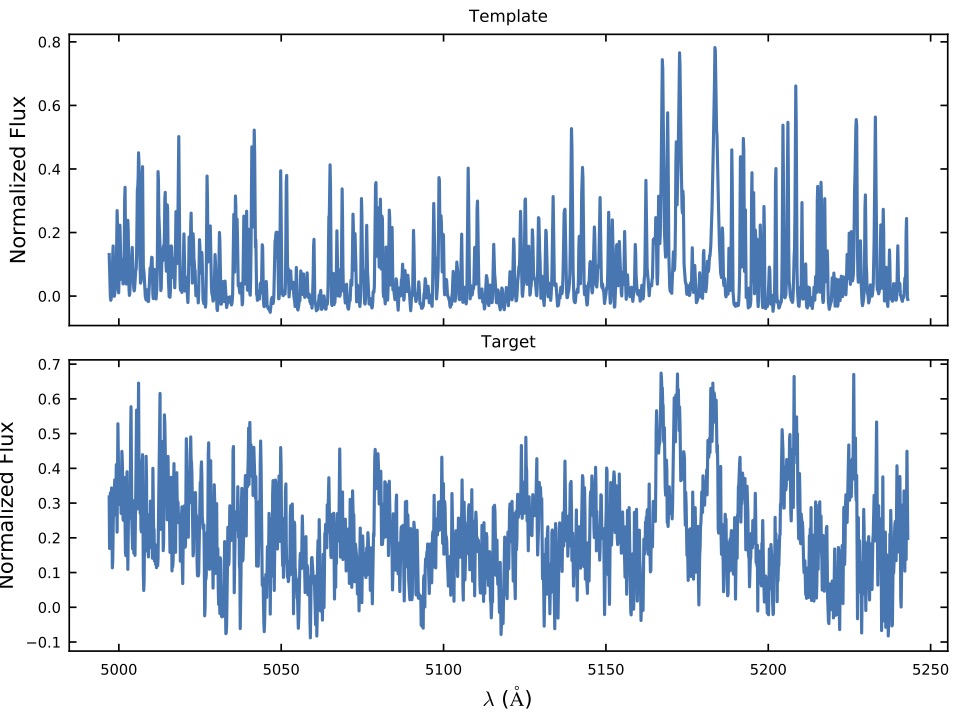
The first is the wavelength region for the template and spectrum which you have used to compute the BF. The spectra are inverted here by convention.

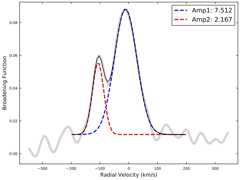
The second is the smoothed BF and the two fit components.

To return their RVs type:

In [8]: tar_spec[tar[0]]['bf_rv']
Out[8]: array([ -11.0376132 , -106.44950092])

The full fit parameters are stored in the tar_spec[tar[0]][‘bf_fits’] array, which can be used to determine the flux ratio of the two stars (division of the BF fit integrals).

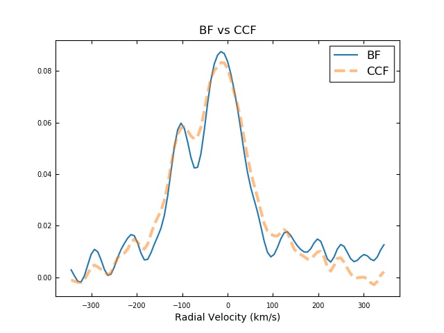
For comparison, the following plot compared the BF above with a CCF computed for the same region. The BF provides a much cleaner separation between the two components.

Parallelizing BF calculations

Why should I parallelize my BF calculations, the worked example above worked just fine without it! Good question. The worked example (Determining RVs of a SB2) used a single order spectra. So it took less than a few seconds to complete all the BF calculations needed. However, you might run into spectra that have 50+ orders. With these spectra, you may want to compare a single template to each order, or even multiple templates to each order. Either way, the amount of computation needed to obtain results has now increased a lot. If you were to do these calculations sequentially (like we did in the SB2 example), it could take a long time. Parallelizing the calculations is our attempt to make your calculation times shorter. We us python’s multipleprocessing library and spawn a new process for each order-template calculation.

Don’t get over-zealous though, parallelizing when you don’t need to will actually slow down calculation times. There is an overhead involved in the spawning of processes, and retrieval of data from each process. So, if you only end up spawning two processes, the time saved on the calculations is overshadowed by the overhead of the multipleprocessing library. But, if you spawn more processes, you would actually see a timing improvement. In general, low-order spectra should be done sequentially whereas high-order spectra should be done parallel-ly.

If you’re stressing about knowing when to use multiple processing and when not too, you can default to using it. In high-order cases, you are getting speed up. In low-order cases, you are being slowed down a little, but since you are still doing little amounts of calculations, the runtime won’t be an issue i.e. it may take 30 seconds sequentially, and 32 seconds in parallel for low-order.

For our example, we will be using fits files from SALT (South Africa Large Telescope). These spectra have 55 orders. For our example we are comparing them against a template spectra found in the file named lte055…. .p.

Our goal here is to establish the radial velocity of the star observed in the SALT spectra. We can do this by calculating a broadening function with each order against the template. You could average out the 55 radial velocity results, one from each order, to find a good estimated value, or you could individually plot them, and put those plots in the same pdf. We will show both.

Download the SALT fits files and ls files from the repo (in the examples folder). Create a new directory and move the downloaded files into it.

Now we will import saphires so we can use its functionality

import saphires as saph

Here we are using the ls file (that splits up the wavelengths of the SALT fits file into sub sections) to create a saphires spectra dictionary. The ls file is created by calling saph.utils.region_select_ms() and doing order-masking (see example in Determining RVs of a SB2). This example refers to order-masking, which the RVs of SB2 example refers to as selecting a region to calculate BF on by clicking the ‘b’ button. We gave you a working ls file, but if you had your own spectra, you would need to go through the order-masking processing yourself.

tar,tar_spec = saph.io.read_ms('./salt1_rb.ls',combine_all=False,header_wave='Single')

Next we read in the template from the pikl file. If we were doing multiple templates, we would have to run the remaining steps for each individual template

temp = saph.io.read_pkl('./lte05500-4.50-0.0.PHOENIX-ACES-AGSS-COND-2011-HiRes_2800-11000_air.p',temp=True)

Now we prepare the spectra with the template spectra

tar_spec = saph.utils.prepare(tar,tar_spec,temp)

Here is where we do the broadening function calculations. There is a multiple_p keyword here that triggers whether the BF calculations happen in a parallel way or not. Currently multiple_p is set to True, meaning the calculations will be done in a parallel fashion. This is going to speed up the calculation process(from 6 minutes to 4.5 minutes on a 4 core Mac Laptop from 2017). If you are ok with the slower version, you can set multiple_p to False. Setting it to False will also prevent lag on your machine while running the calculations.

tar_spec = saph.bf.compute(tar,tar_spec,vel_width=400,multiple_p = True)

This is where we analyze the BF data. When the keyword single_plot is set to True, a pdf will be generated with all the results(plots) from each order. With text_out = True, we generate a text file with the results of our bf calculations. When text_out is True, you can also set text_name to a specific file name, if you leave the text_name it will still make a file, just with a default file name of bf_text.dat

tar_spec = saph.bf.analysis(tar,tar_spec,R=50000,single_plot=True,text_out = True,text_name = "file_name.txt")