Broadening Function Walkthrough

Graphical Representations

Embedded in the discussion below are some slides that graphically describe spectral-line broadening functions.

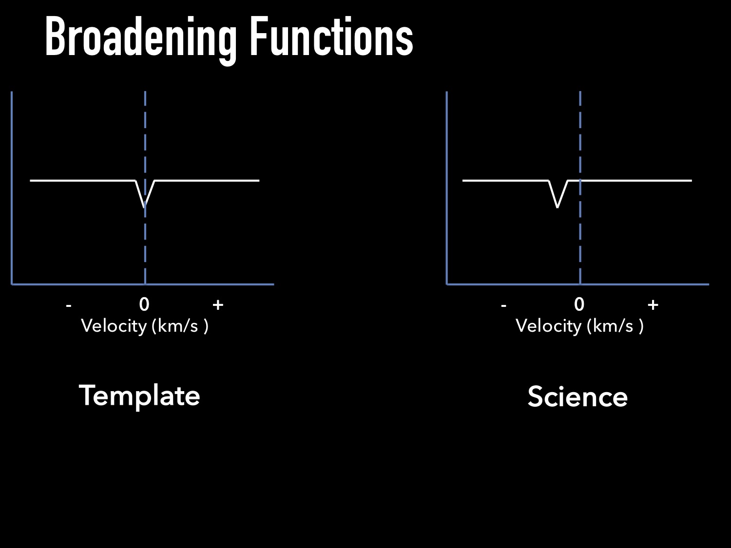
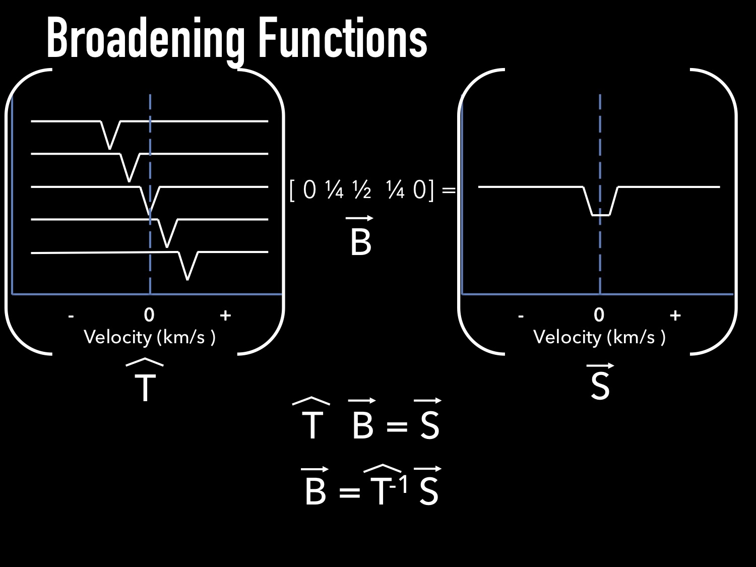
As with most radial velocity (RV) measurement techniques, you need a Template spectrum. In the graphical representation below, our template (left) is narrow-lined, at zero velocity, and for the sake of this example, one absorption line. The star we observe, the Science spectrum (right), is an exact match to the template but with an RV shift.

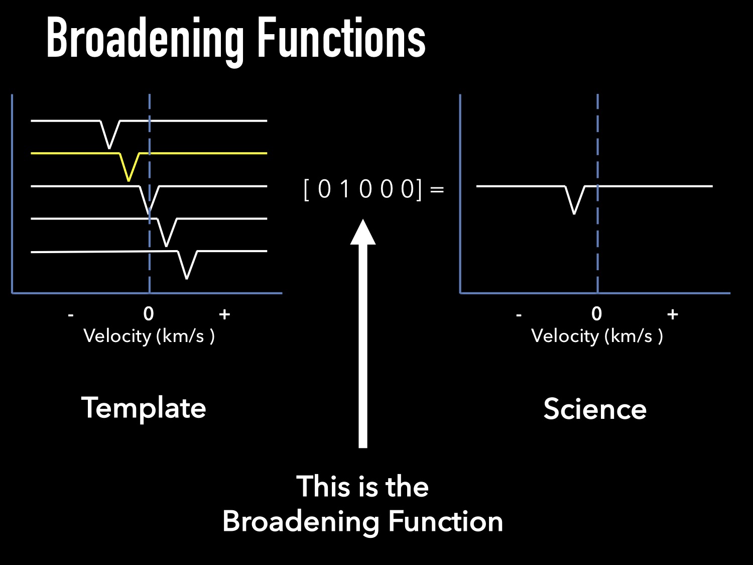
The broadening function can be described as the function that you need to convolve the template spectrum with to return the observed spectrum. Convolutions are typically described by sliding integrals [1], but I find that definition to be, well, convoluted (apologies). A more useful way to think about them, especially in terms of how they are actually computed, is as a linear combination of template spectra at different RV shifts. In the next figure, the same template is reproduced at many velocity shifts, and a linear combination of these templates can be shown to match the observed spectrum. In this pedestrian example, a simple RV shift is recreated by a linear combination of one specific template. That linear combination is the broadening function, with the array you see below plotted as the y-axis and the RV shift as the x-axis (see below). In practice, the velocity shifts are set by the wavelength spacing of the template and observed spectrum.

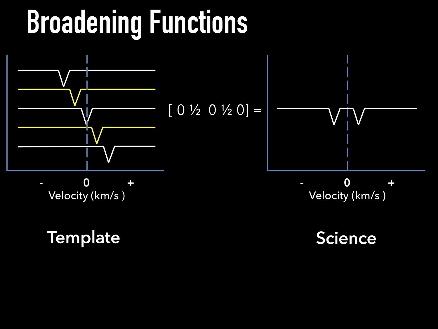
In this example, our observed spectrum is an equal-mass, double-lined spectroscopic binary (SB2). Here the BF corresponds to a linear combination of two template spectra at different RVs.

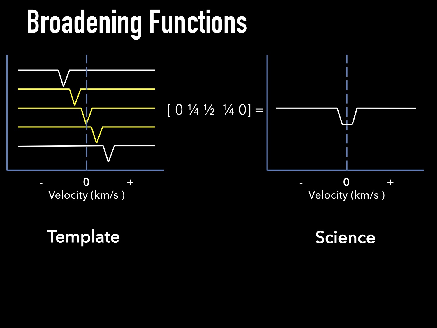
In this example, we have a mock rotationally broadened star that requires three adjacent templates.

These graphical representations are all well and good, but how to we actually solve for the BF? In the next figure we turn these into math objects. The shifted templates become a matrix, T, and the BF and Science spectrum become the B and S arrays, respectively. If T were an invertible matrix, we could solve for B with simple matrix algebra. In practice, T is not invertible, so we rely on singular-value decomposition [2] to decompose T in to other matrices that are invertible in order to solve for B.

Smoothing

As noted on the Introduction page, the raw BF has to be smoothed in order to be useful. As implemented here, the smoothing is set by the resolution (R) you set in the saphires.bf.analysis function. This is because the best place to start is with your instrument’s spectral resolution. You have a little bit of room to make some choices here on what level you decide to smooth to, but there are some important things to keep in mind. Low S/N spectra require additional smoothing (lower R) to make a decent fit. This is fine for RVs but if you want to recover the intrinsic line profile of your star, you need to smooth by the line width of your template. If you’re using a narrow-lined, empirical template taken with the same instrument (where the spectral lines are unresolved) the instrumental resolution is the correct choice. If the template is synthetic you will want to smooth by the template’s resolution.

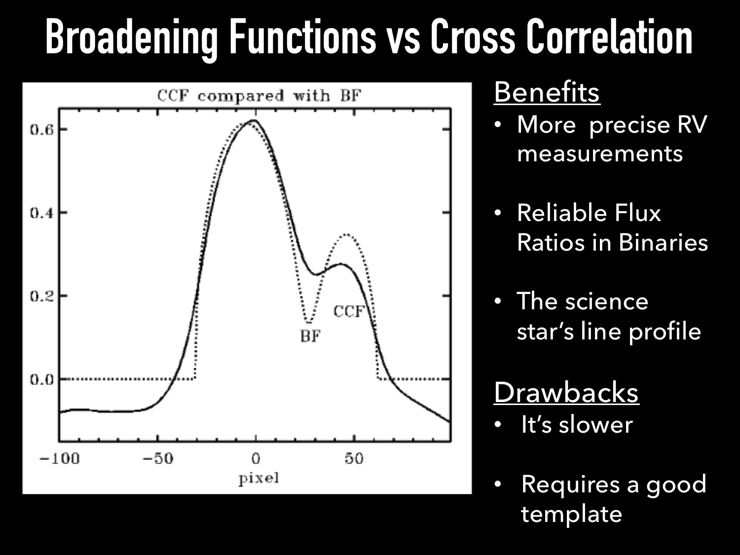
A smoothed BF computed from a synthetic double-lined, rapidly-rotating binary system is shown below, and compared with a CCF.

[1]	Convolution

[2]

SVD